Ⅰ Abstract
Point cloud completion aims to predict a complete shape in high accuracy from its partial observation. However, previous methods usually suffered from discrete nature of point cloud and unstructured prediction of points in local regions, which makes it hard to reveal fine local geometric details on the complete shape. To resolve this issue, we propose SnowflakeNet with Snowflake Point Deconvolution (SPD) to generate the complete point clouds. The SnowflakeNet models the generation of complete point clouds as the snowflake-like growth of points in 3D space, where the child points are progressively generated by splitting their parent points after each SPD. Our insight of revealing detailed geometry is to introduce skip-transformer in SPD to learn point splitting patterns which can fit local regions the best. Skip-transformer leverages attention mechanism to summarize the splitting patterns used in the previous SPD layer to produce the splitting in the current SPD layer. The locally compact and structured point cloud generated by SPD is able to precisely capture the structure characteristic of 3D shape in local patches, which enables the network to predict highly detailed geometries, such as*Equal contribution. This work was supported by National Key R&D Program of China (2020YFF0304100), the National Natural Science Foundation of China (62072268), and in part by Tsinghua-Kuaishou Institute of Future Media Data. The corresponding author is Yu-Shen Liu.smooth regions, sharp edges and corners. Our experimental results outperform the state-of-the-art point cloud completion methods under widely used benchmarks.
文章指出以往的点云补全方法受到: 1)点云离散特性 2)点的非结构化预测 的影响,导致很难揭示出局部几何特性信息。因此文章提出了附带SPD(Snowflake Point Deconvolution)模块的SnowfakeNet网络结构;SnowflakeNet 将完整点云的生成建模为 3D 空间中点的雪花状生长。同时提出了SPD模块中的skip-transformer来学习具体的几何信息。
Ⅱ Introduction:
现阶段存在的办法如:“hierarchical rooted tree structure”、“assume a specific topology”等受制于点云的离散特性与非结构化的点预测,难以捕获局部特征如平滑区域、尖锐边缘和角落,如上图所示。
Contributions:
- 我们提出了一种新的SnowflakeNet来补全点云。与之前的局部无组织的方法相比,SnowflakeNet可以将完整点云的生成过程解释为显式和结构化的局部模式生成,大大提高了三维形状补全的性能。
- 提出了新的雪花点反卷积( SPD )来逐步增加点的数量。它将父点生成子点的过程重新表述为雪花生长过程,父点特征中嵌入的形状特征通过逐点分裂 ( pointwise splitting ) 操作被子点提取并继承。
- 引入了skip-transformer来学习SPD中的分裂模式。它学习子点和父点之间的形状上下文和空间关系。skip-transformer鼓励SPD产生局部结构化和紧凑的点排布,并捕捉局部面片中三维表面的结构特征。
Ⅲ SnowflakeNet
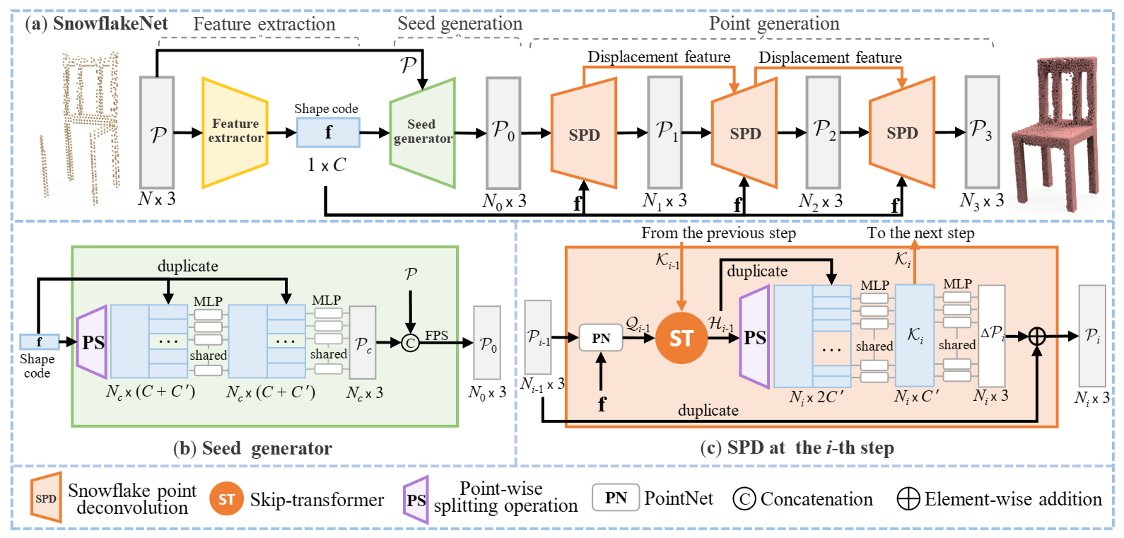
SnowflakeNet的整体架构如上所示,它由三个模块组成:特征提取、种子生成和点生成。
3.1 Overview
a. Feature extraction module
特征提取器提取一个大小为1 × C的形状编码f,该编码捕获目标形状的全局结构和细节局部模式。
具体采用了PointNet++中的三层集合抽象来聚合从局部到全局的点特征,并使用Point transformer来合并局部形状上下文。
...
self.sa_module_1 = PointNet_SA_Module_KNN(512, 16, 3, [64, 128], group_all=False, if_bn=False, if_idx=True)
self.transformer_1 = Transformer(128, dim=64)
self.sa_module_2 = PointNet_SA_Module_KNN(128, 16, 128, [128, 256], group_all=False, if_bn=False, if_idx=True)
self.transformer_2 = Transformer(256, dim=64)
self.sa_module_3 = PointNet_SA_Module_KNN(None, None, 256, [512, out_dim], group_all=True, if_bn=False)
...
l1_xyz, l1_points, idx1 = self.sa_module_1(l0_xyz, l0_points)  # (B, 3, 512), (B, 128, 512)
l1_points = self.transformer_1(l1_points, l1_xyz)
l2_xyz, l2_points, idx2 = self.sa_module_2(l1_xyz, l1_points)  # (B, 3, 128), (B, 256, 512)
l2_points = self.transformer_2(l2_points, l2_xyz)
l3_xyz, l3_points = self.sa_module_3(l2_xyz, l2_points)  # (B, 3, 1), (B, out_dim, 1)
...
b. Seed generation module
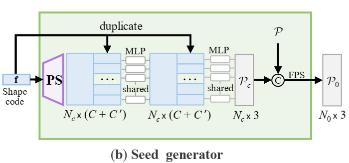
种子生成器的目标是生成一个粗略但完整的点云P0,其大小为N0 × 3,能够捕获目标形状的几何和结构。
利用提取的形状编码f,种子生成器首先通过逐点分裂操作(point-wise splitting operation ,即 PS)产生同时捕获现有结构和缺失结构的点特征。然后,通过多层感知器( MLP )将点特征与形状编码集成,生成尺寸为Nc × 3的粗略点云Pc。然后,沿用之前的方法,将Pc与输入点云P进行拼接合并,再通过最远点采样( FPS )将合并后的点云降采样到P0。在本文中,我们通常设置Nc = 256和N0 = 512,其中稀疏点云P0足以表示底层形状。P0将作为点生成模块的种子点云。
...
self.ps = nn.ConvTranspose1d(dim_feat, 128, num_pc, bias=True)
self.mlp_1 = MLP_Res(in_dim=dim_feat + 128, hidden_dim=128, out_dim=128)
self.mlp_2 = MLP_Res(in_dim=128, hidden_dim=64, out_dim=128)
self.mlp_3 = MLP_Res(in_dim=dim_feat + 128, hidden_dim=128, out_dim=128)
self.mlp_4 = nn.Sequential(nn.Conv1d(128, 64, 1),nn.ReLU(),nn.Conv1d(64, 3, 1))
...
x1 = self.ps(feat)  # (b, 128, 256)
x1 = self.mlp_1(torch.cat([x1, feat.repeat((1, 1, x1.size(2)))], 1))
x2 = self.mlp_2(x1)
x3 = self.mlp_3(torch.cat([x2, feat.repeat((1, 1, x2.size(2)))], 1))  # (b, 128, 256)
completion = self.mlp_4(x3)  # (b, 3, 256)
...
c. Point generation module
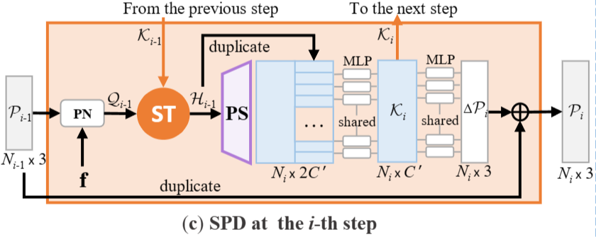
点生成模块由3个雪花点反卷积( SPD )步骤组成,每个步骤以上一步点云为输入,通过上采样因子(用r1 , r2和r3表示)对其进行分割,得到P1、P2、P3,点尺寸分别为N1 × 3、N2 × 3、N3 × 3。SPDs协作为每个种子点生成符合局部模式的有根树结构。
...
b, _, n_prev = pcd_prev.shape
feat_1 = self.mlp_1(pcd_prev)
feat_1 = torch.cat(...)//维度扩充
Q = self.mlp_2(feat_1)
H = self.skip_transformer(pcd_prev, K_prev if K_prev is not None else Q, Q)
feat_child = self.mlp_ps(H) //反卷积前conv一下
feat_child = self.ps(feat_child)  # (B, 128, N_prev * up_factor)
H_up = self.up_sampler(H)//疑问:unsample与convtrans
K_curr = self.mlp_delta_feature(torch.cat([feat_child, H_up], 1))
delta = self.mlp_delta(torch.relu(K_curr)) //PCN
if self.bounding:
    delta = torch.tanh(delta) / self.radius**self.i  # (B, 3, N_prev * up_factor)
pcd_child = self.up_sampler(pcd_prev)
pcd_child = pcd_child + delta
...
3.2 Snowflake Point Deconvolution (SPD)
a. Motivation
为实现 1)捕捉局部几何模式 2)点分裂特征传递 两个任务,自注意力机制是一个很好的解决方案;但是transformer只考虑当前步骤中的上下文,而忽略了历史分裂信息,所以提出了skip-transformer来实现SPD之间的协作。
而跳跃变压器(skip-transformer)得益于注意力机制,能够很好地捕获局部上下文,同时在连续的SPD中也能调整分裂模式。在捕获到局部几何模式后,可以通过先复制父特征再添加变化来获得子特征。现有的方法通常采用基于折叠的策略来获得变化,用于学习重复点的不同位移。然而,折叠操作对每个父点采样相同的二维网格,忽略了父点包含的局部形状特征。相比之下,SPD通过逐点分裂操作获得变化量,充分利用父点中的几何信息,增加符合局部模式的变化量。
b. Point-wise splitting operation
逐点分裂操作旨在为每个 $h_{j}^{i-1}\in H_{i-1}$ 生成多个子点特征。 它是一种特殊的一维反卷积策略,其中核大小和步长等于ri。
实际上,每个 $\begin{aligned}h_j^{i-1}\in H_{i-1}\end{aligned}$ 共享同一组内核,并以逐点方式产生多个子点特征。为清楚起见我们将 $h_j^{i-1}$ 的第m个logit 表示为 $h_{j,m}^{i-1}$ ,其对应的内核用 $K_{m}$ 表示。从技术上讲,$K_{m}$ 是个大小为rix C’的矩阵, $K_{m}$ 的第k行表示为 $K_{m,k}$ ,第k个子点特征 $g_{j,k}$ 由下式给出 \(\mathbf{g}_{j,k}=\sum_{m}h_{j,m}^{i-1}\mathbf{k}_{m,k}\) 此外,逐点分裂操作对于上采样点是灵活的。
- 当ri = 1 时,SPD可以将上一步的点移动到更好的位置;
- 当ri > 1 时,它用于将点数扩大 ri 倍。
c. Collaboration between SPDs
文章采用了三个SPD来生成完整的点云。首先设置上采样因子r1 = 1来明确地重新排列种子点位置。然后,我们设定r2 > 1和r3 > 1为P1中的每个点生成一棵结构化树。SPD之间的协作对于树的协调生长至关重要,因为上一个分裂步骤的信息可以用来指导当前步骤。
此外,有根树的生长还应该捕获local patches的特征,以防止它们重叠。为了实现这一点,文章提出了一种Skip-Transformer作为SPD之间的协作单元。
3.3 Skip-Transformer
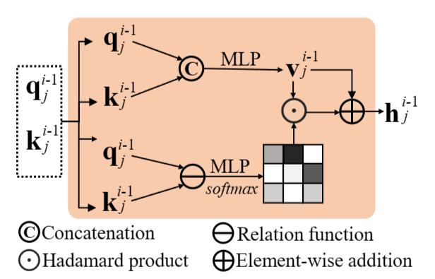
Skip-Transformer以每个点的特征 $q_{j}^{i-1}$ 作为输入,并与上一步的位移特征 $K_{i}^{i-1}$ 相结合产生形状上下文特征 $h_{j}^{i-1}$ ,其由下式给出: \(\mathbf{h}_{j}^{i-1}=\mathrm{ST}(\mathbf{k}_{j}^{i-1},\mathbf{q}_{j}^{i-1})\) 上图所示为skip-transformer的结构。引入skip-transformer来学习和细化父点和子点之间的空间上下文,其中”跳跃”一词表示来自上一层的位移特征和当前层的点特征之间的联系。
跳跃变压器首先将它们串联起来。然后,将拼接后的特征送入MLP,MLP生成向量 $V_{j}^{i-1}$ 。其中,$V_{j}^{i-1}$作为值向量,包含了之前的点分裂信息。 为了进一步将局部形状上下文聚合为 $V_{j}^{i-1}$ ,跳跃变压器使用 $q_{j}^{i-1}$ 作为查询,$K_{j}^{i-1}$ 作为密钥来估计注意力向量 $a_{j}^{i-1}$ ,其中 $a_{j}^{i-1}$ 表示当前分裂应该给予前一个分裂多少注意力。为了使跳跃变压器能够专注于局部模式,我们计算每个点与其k近邻( k-NN)之间的注意力向量。k - NN策略也有助于降低计算成本。 具体来说,给定第个点特征 $q_{j}^{i-1}$ ,$q_{j}^{i-1}$与第k个近邻的位移特征{$K_{j,l}^{i-1}$|L =1,2,.,k}之间的注意力向量 $a_{j,l}^{i-1}$ 可计算如下:
其中⊕表示逐元的加法, ⊙ 为Hadamard Product(哈达玛乘积);注意第一个SPD没有先前的位移特征。
class SkipTransformer(nn.Module):
    def __init__(self, in_channel, dim=256, n_knn=16, pos_hidden_dim=64, attn_hidden_multiplier=4):
        super(SkipTransformer, self).__init__()
        self.mlp_v = MLP_Res(in_dim=in_channel*2, hidden_dim=in_channel, out_dim=in_channel)
        self.n_knn = n_knn
        self.conv_key = nn.Conv1d(in_channel, dim, 1)
        self.conv_query = nn.Conv1d(in_channel, dim, 1)
        self.conv_value = nn.Conv1d(in_channel, dim, 1)

        self.pos_mlp = nn.Sequential(
            nn.Conv2d(3, pos_hidden_dim, 1),
            nn.BatchNorm2d(pos_hidden_dim),
            nn.ReLU(),
            nn.Conv2d(pos_hidden_dim, dim, 1)
        )

        self.attn_mlp = nn.Sequential(
            nn.Conv2d(dim, dim * attn_hidden_multiplier, 1),
            nn.BatchNorm2d(dim * attn_hidden_multiplier),
            nn.ReLU(),
            nn.Conv2d(dim * attn_hidden_multiplier, dim, 1)
        )

        self.conv_end = nn.Conv1d(dim, in_channel, 1)

    def forward(self, pos, key, query, include_self=True):
        """
        Args:
            pos: (B, 3, N)
            key: (B, in_channel, N)
            query: (B, in_channel, N)
            include_self: boolean

        Returns:
            Tensor: (B, in_channel, N), shape context feature
        """
        value = self.mlp_v(torch.cat([key, query], 1))
        identity = value
        key = self.conv_key(key)
        query = self.conv_query(query)
        value = self.conv_value(value)
        b, dim, n = value.shape

        pos_flipped = pos.permute(0, 2, 1).contiguous()
        idx_knn = query_knn(self.n_knn, pos_flipped, pos_flipped, include_self=include_self)

        key = grouping_operation(key, idx_knn)  # b, dim, n, n_knn
        qk_rel = query.reshape((b, -1, n, 1)) - key

        pos_rel = pos.reshape((b, -1, n, 1)) - grouping_operation(pos, idx_knn)  # b, 3, n, n_knn
        pos_embedding = self.pos_mlp(pos_rel)

        attention = self.attn_mlp(qk_rel + pos_embedding)  # b, dim, n, n_knn
        attention = torch.softmax(attention, -1)

        value = value.reshape((b, -1, n, 1)) + pos_embedding  #

        agg = einsum('b c i j, b c i j -> b c i', attention, value)  # b, dim, n
        y = self.conv_end(agg)

        return y + identity
3.4 Training Loss
文章使用Chamfer distance (CD) 作为主要损失函数。为了明确约束种子生成和随后的拆分过程中生成的点云,我们将ground truth点云下采样到与 {Pc, P1, P2, P3} 相同的采样密度,其中我们将四个 CD 损失的总和定义为完成损失,用 Lcompletion 表示。此外,我们还利用Cycle4Completion中的部分匹配损失来保留输入点云的形状结构。这是一个单向约束,旨在匹配一个形状,而不约束相反的方向。由于部分匹配损失只需要输出点云部分匹配输入,我们将其作为保留损失Lpreservation保存,总训练损失表示为: \(\mathcal{L}=\mathcal{L}_\text{completion}+\lambda\mathcal{L}_\text{preservation}\)
\[{\cal L}_{\mathrm{CD}_{2}}({\cal X},{\cal Y})=\sum_{\mathbf{x}\in{\cal X}}\min_{\mathbf{y}\in{\cal Y}}\|\mathbf{x}-\mathbf{y}\|_{2}+\sum_{\mathbf{y}\in{\cal Y}}\operatorname*{min}_{\mathbf{x}\in{\cal X}}\|\mathbf{y}-\mathbf{x}\|_{2}\]同时,作者也效仿 MSN和 SpareNet将地球自转距离( Earth Mover ‘ s Distance,EMD )作为训练损失,其定义如下:
\[\mathcal{L}_{\mathrm{EMD}}=\min_{\phi:\mathcal{X}\rightarrow\mathcal{Y}}\sum_{x\in\mathcal{X}}\|\mathbf{x}-\phi(\mathbf{x})\|_{2}\]Ⅳ Experiments
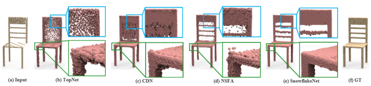
To fully prove the effectiveness of our SnowflakeNet, we conduct comprehensive experiments under two widely used benchmarks: PCN [57] and Completion3D [43], both of which are subsets of the ShapeNet dataset. The experiments demonstrate that our method has superiority over the state-of-the-art point cloud completion methods.
4.1 Evaluation
Omitted
4.2 Ablation studies
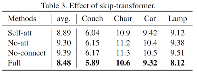
a. Effect of skip-transformer.
- Self-att 变体将 skip-transformer 中的转换器机制替换为自注意力机制,其中输入是当前层的点特征。
- No-att 变体从 skip-transformer 中删除了转换器机制,其中 SPD 前一层的特征直接添加到当前 SPD 层的特征中。
- No-connect 变体从 SPD 层中删除了整个 skip-transformer,因此 SPD 层之间没有建立特征连接。
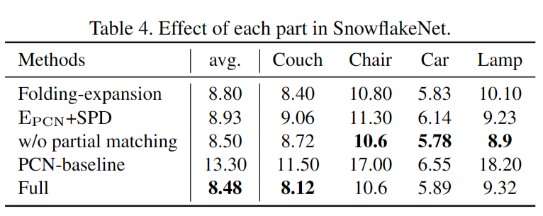
b. Effect of each part in SnowflakeNet.
(1)The Folding expansion变化用基于折叠的特征扩展方法取代了逐点分裂操作,其中特征重复多次并与二维码字连接,以增加点特征的数量。
(2) EPCN+SPD 变化:采用 PCN 编码器和我们的 SnowflakeNet 解码器。
(3) w/o partial matching变化去除了部分匹配损失。
(4) PCN-baseline 是原始 PCN 方法的性能 ,它在消融研究的相同设置下训练和评估
Ⅴ Improvement of TPAMI Version
与发布在ICCV上的版本相比(即本BLOG版本),该工作发布在TPAMI上的版本,主要增加了SnowflakeNet在其他点云处理任务上的Evaluation,同时增加了在ShapeNet-34/21数据集上补全的Evaluation。
In addition to point cloud completion, we further generalize SPD to more tasks related to point cloud generation. With a few network arrangements, SPD can be well applied to multiple point cloud generation scenarios. Comprehensive experiments are conducted to verify the effectiveness and generation ability of SPD.
5.1 Evaluation on the ShapeNet-34/21 Dataset
Omitted.
5.2 Extension to Real-World Scenarios
为了评估SnowflakeNet在现实场景中的泛化能力,文章在KITTI基准、和ScanNet Chairs上进行了实验。
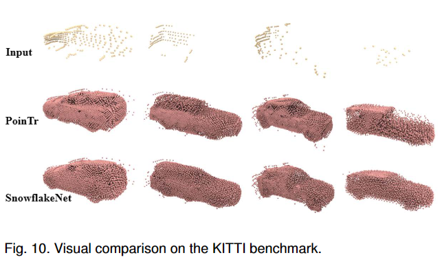
a. Extension to the KITTI benchmark
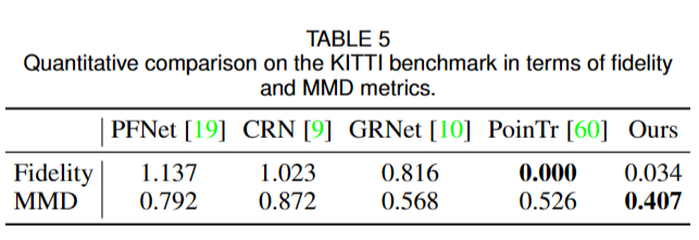
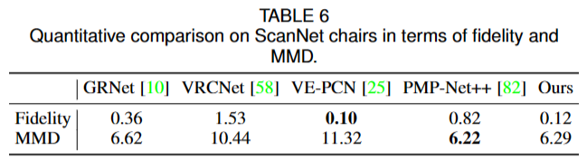
Fidelity是指生成点云与真实点云之间的重叠程度,也就是生成点云覆盖了多少真实点云,取值范围在0到1之间。MMD是指生成点云与真实点云之间的最小匹配距离,也就是生成点云与真实点云之间的距离越小,MMD值越小,生成点云质量越好。
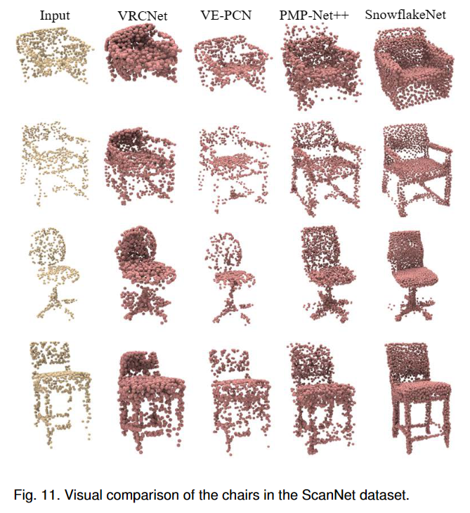
b. Extension to the ScanNet
为了进一步评估稀疏点云补全在现实场景中的性能,文章在Completion3D数据集上使用SnowflakeNet的预训练模型,并在ScanNet数据集中的椅子实例上评估其性能,而无需进行微调。
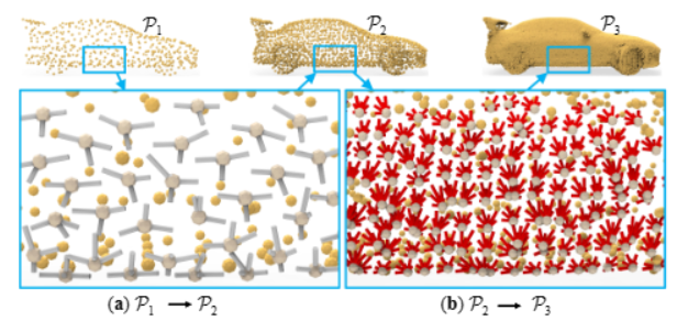
5.3 Point Cloud Auto-Encoding
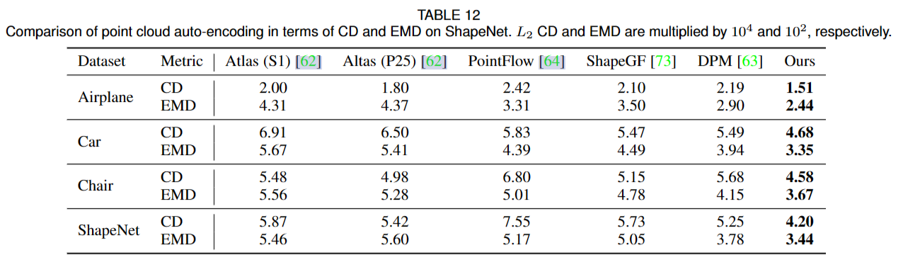
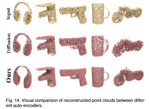
点云自编码的任务旨在从编码后精简的样本中中重建点云。由于它严重依赖于解码器的生成能力,我们在点云自编码中使用 SnowflakeNet 的解码部分来评估雪花点反卷积的生成能力。
使用“Diffusion Probabilistic Models for 3D Point Cloud Generation”同样的设置,使用ShapaNet数据集。采用常用的Chamfer distance(CD)和Earth Mover’s distance(EMD)作为评价指标。
\(\mathcal{L}_{recon}=\sum_{i\in\{0,2\}}\mathcal{L}_{\mathrm{CD}_2}(\mathcal{P}_i,\mathcal{P}_i^{'})+\mathcal{L}_{\mathrm{EMD}}(\mathcal{P}_i,\mathcal{P}_i^{'})\)
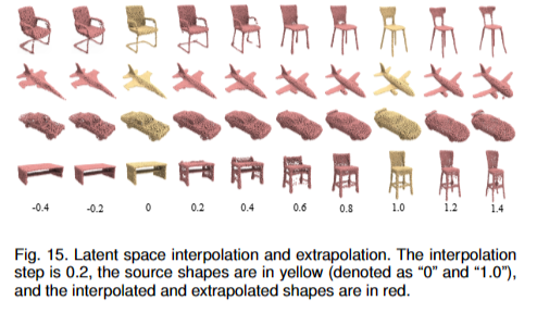
文章在图15中可视化了潜在代码之间的interpolation and extrapolation,其中源形状为黄色,interpolation 形状和extrapolation形状为红色。图 15 显示 即使过渡在不同类别之间(最后一行的桌子和椅子)SnowflakeNet 的输出能够根据潜在插值和外推平滑地传输。
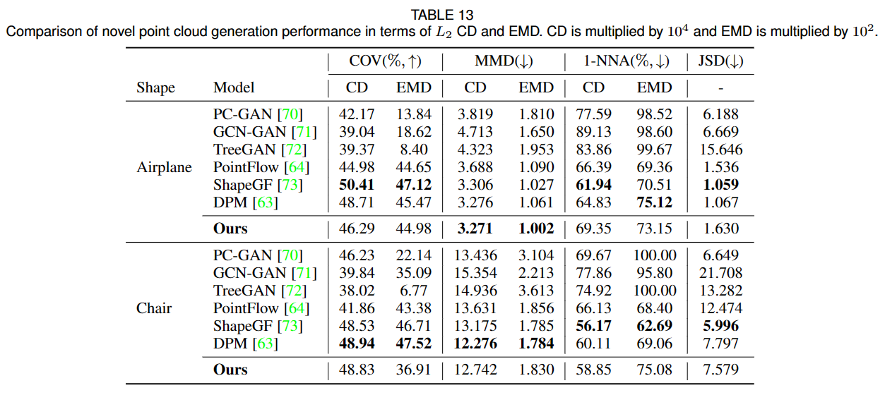
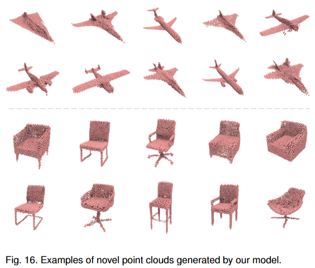
5.4 Novel Shape Generation
点云生成任务。文章采用DPM的方法并在 ShapeNet 数据集上进行实验。文章使用覆盖率分数 (the coverage score, COV)、最小匹配距离 (MMD)、1-NN 分类器准确度 (1-NNA) 和 Jenson-Shannon 散度 (JSD)作为Metric。
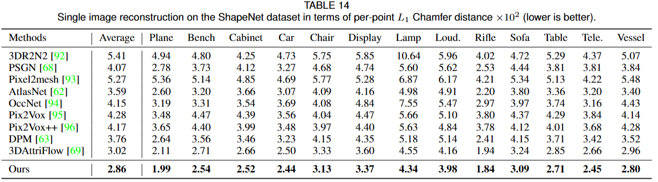
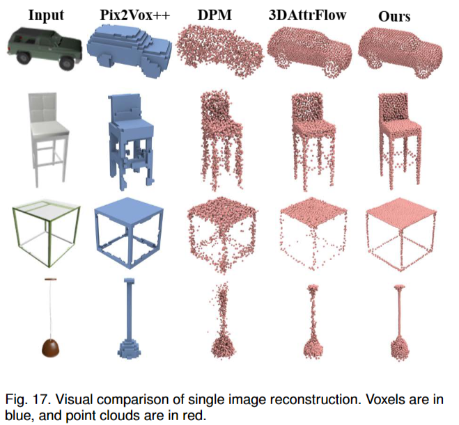
5.5 Single Image Reconstruction
单幅图像重建(SVR)的任务,其目标是从图像中重建点云。
使用ShapeNet数据集,在训练时跟踪验证集上的损失以确定何时停止训练。采用 L1 Chamfer distance (CD) 来评估所有对应物之间的生成质量。
\(\mathcal{L}_{\mathrm{SVR}}=\sum_{i\in\{0,2\}}\mathcal{L}_{\mathrm{CD}_1}(\mathcal{P}_i,\mathcal{P}_i^i)\)
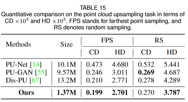
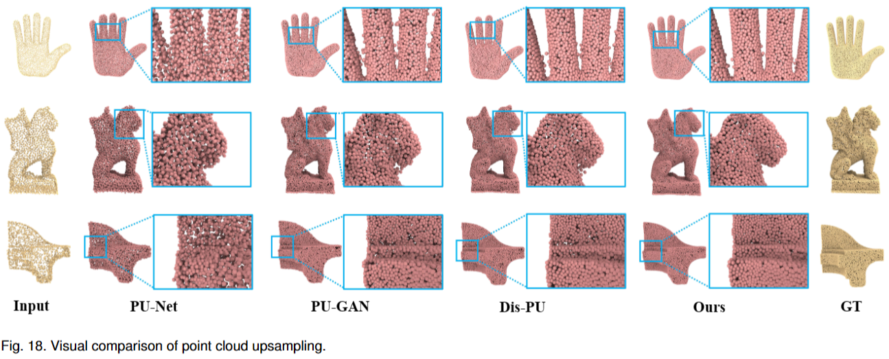
5.6 Point Cloud Upsampling
给定一个稀疏、噪声和非均匀的点云,点云上采样的任务需要对密集和均匀的点云进行上采样和生成。因为它也是一个生成问题,在本节中,我们将雪花点反卷积 (SPD) 扩展到点云上采样。
使用PU-GAN提供的数据集,由于输入点云的质量对点云上采样的性能影响很大,文章分别采用了FPS和RS两种方法获取输入点云。为了减轻随机抽样带来的不稳定性,文章在随机抽样五次下重复测试,并将平均分数作为最终结果。
我们使用L2 Chamfer distance(CD)和Hausdorff距离(HD)作为评估指标
\[\mathcal{L}_{\mathrm{SVR}}=\sum_{i\in\{0,2\}}\mathcal{L}_{\mathrm{CD}_1}(\mathcal{P}_i,\mathcal{P}_i^i)\]Hausdorff距离是一种衡量两个点云之间的相似度的指标,它是两个点云之间最长距离的最小值。具体来说,它是指在一个点云中的每个点,找到距离其最近的另一个点云中的点,然后取这些距离的最大值。因此,Hausdorff距离可以衡量两个点云之间的形状差异和变形程度。在计算机视觉和计算机图形学中,Hausdorff距离常常被用来评估3D模型之间的相似度和形状变化。